Running An Analysis Of Variance on Gapminder Data

In this post I run an analysis of variance (ANOVA) on the Gapminder dataset. Because the Gapminder data contains mainly continous values and not categorical ones, I had to create categorical values using the “qcut” function from Python’s Pandas library. Let’s take a look at the code used to load, preprocess, and bin the data.

import statsmodels.formula.api as smf
import statsmodels.stats.multicomp as multi
import pandas as pd

# check for missing data
def check_missing(dataframe, cols):

    for col in cols:
       print("Column {} is missing:".format(col))
       print((dataframe[col].values == ' ').sum())
       print()

# convert to numeric
def to_numeric(dataframe, cols):

    for col in cols:
        dataframe[col] = dataframe[col].convert_objects(convert_numeric=True)

# check frequency distribution
def freq_dist(dataframe, cols, norm_cols):

    for col in cols:
        print("Fred dist for: {}".format(col))
        count = dataframe[col].value_counts(sort=False, dropna=False)
        print(count)

    for col in norm_cols:
        print("Fred dist for: {}".format(col))
        count = dataframe[col].value_counts(sort=False, dropna=False, normalize=True)
        print(count)


df = pd.read_csv("gapminder.csv")

#print(dataframe.head())
#print(df.isnull().values.any())

cols = ['lifeexpectancy', 'breastcancerper100th', 'suicideper100th']
norm_cols = ['internetuserate', 'employrate']

df2 = df.copy()

#check_missing(df, cols)
#check_missing(df, norm_cols)

to_numeric(df2, cols)
to_numeric(df2, norm_cols)

#freq_dist(df2, cols, norm_cols)

def bin(dataframe, cols):

    for col in cols:
        new_col_name = "{}_bins".format(col)
        dataframe[new_col_name] = pd.qcut(dataframe[col], 10, labels=["1=10%", "2=20%", "3=30%", "4=40%", "5=50%",
                                                                     "6=60%", "7=70%", "8=80", "9=90%", "10=100%"])

df3 = df2.copy()
#bin(df3, cols)
bin(df3, norm_cols)

I’ll run an ANOVA on the life expectancy data and binned internet user rate data. I’ll make an ANOVA frame and another frame to check mean and standard deviation on. I then fit the stats OLS model and print out the results, along with the mean and standard dev to get more context.

anova_frame = df3[['lifeexpectancy', 'breastcancerper100th', 'suicideper100th',
                   'internetuserate_bins', 'employrate_bins']].dropna()

relate_frame = df3[['lifeexpectancy', 'internetuserate_bins']]

anova_model = smf.ols(formula='lifeexpectancy ~ C(internetuserate_bins)', data=anova_frame).fit()
print(anova_model.summary())
mean = relate_frame.groupby("internetuserate_bins").mean()
sd = relate_frame.groupby("internetuserate_bins").std()

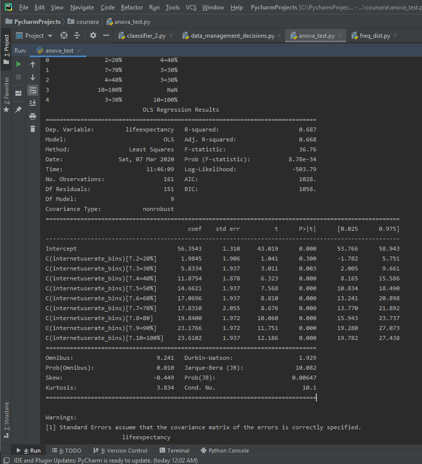
Here’s the results for the OLS ANOVA.

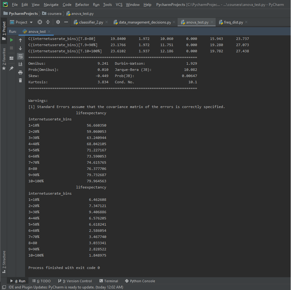
Here’s the mean and standard dev for the internet use rate and life expectancy.

The F-Score is 36.76, while the P-Value is 8.78e-34, which is a very small P-value. This seems to be a significant relationship. There are 10 different categories in the binned Internet Use Rate variables, and since the P-value is small enough to be significant we want to run a post-hoc comparison.

Here’s the code to run the multi-comparison.

multi_comp = multi.MultiComparison(anova_frame["lifeexpectancy"], anova_frame["internetuserate_bins"])
results = multi_comp.tukeyhsd()
print(results)

And here’s the results for the multi-comparison.

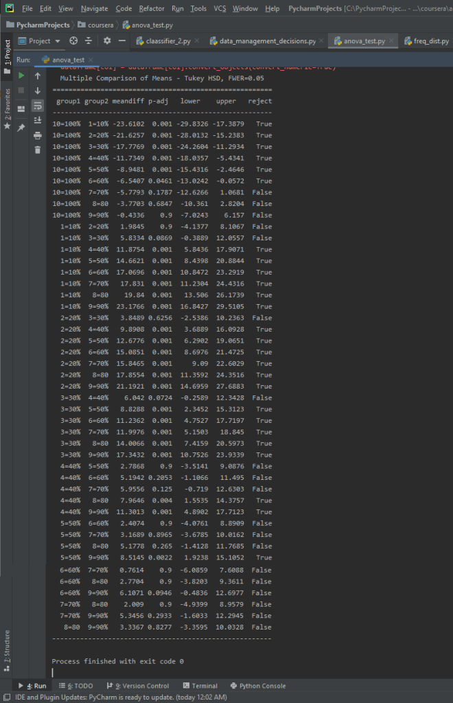
We can see that there are significant differences, and that we can reject the null hypothesis for the majority of these class/group differences.