
Training a deep neural network can take a substantial amount of time. Not only will you often need to create a model architecture and train the model, but you’ll likely need to tweak the model to get optimal performance out of the model. This can drastically increase the amount of time needed to train a model. In order to speed up the process of training and deploying a model, a technique called transfer learning is used. Transfer learning lets you take a model architecture and reuse it, potentially using the same weights the model has learned before.
You can take a model architecture than has already been defined and reuse it, either using the same weights or retaining the model and just using the architecture. You can also do something in between and retrain just some of the layers of the architecture. This blog post will demonstrate the creation of a deep learning model in Keras and then demonstrate how the model can be reused on another, similar dataset.
I’ll be creating a Convolutional Neural Network in Keras, saving the model and then reapplying it to another image classification problem. We’ll be using the Chest X-Ray Image Dataset, available HERE for this project. I’ll be splitting up the training data folder into a training and validation set. We’ll use this initial dataset for the training and testing of the model. After that, I’ll apply some perturbations to the test dataset to simulate image corruption and transfer the pre-trained model over, retraining it to classify the damaged images.
To begin with, here are the imports we’ll need.
from keras.preprocessing.image import ImageDataGenerator
import keras
from keras.models import Sequential
from keras.layers import Dense, Conv2D, BatchNormalization, Dropout, MaxPooling2D, Flatten, Activation
from keras.callbacks import ModelCheckpoint, ReduceLROnPlateau, EarlyStopping
import matplotlib.pyplot as plt
Now we’ll define some variables we’ll need, as well as handle different possible input specifications for our model. Some models want the channels listed first, others don’t.
batch_size = 16
im_height = 150
im_width = 150

# handling the different possible input shapes for the model

if keras.backend.image_data_format() == 'channels_first':
    inp_shape = (3, im_width, im_height)
else:
    inp_shape = (im_width, im_height, 3)
We’ll now want to specify the directories and use the ImageDataGenerator to get the image data from the directories. After that, we’ll use the generators and make iterables from them using flow_from_directory.
train_dir = "chest_xray/train"
val_dir = "chest_xray/val"
test_dir = "chest_xray/test"

# generate the data for both training and validation data
# when we instantiate the data generator we pass in transformations to use
# rescaling and flipping here

train_1_datagen = ImageDataGenerator(rescale=1. / 255)

train_2_datagen = ImageDataGenerator(rescale=1. /255, shear_range=0.2, zoom_range=0.2, horizontal_flip=True, rotation_range=30,
                                     width_shift_range=0., channel_shift_range=0.9, brightness_range=[0.5, 1.5])

test_datagen = ImageDataGenerator(rescale=1. /255)

test_datagen_2 = ImageDataGenerator(rescale=1. /255, shear_range=0.2, zoom_range=0.2, horizontal_flip=True, rotation_range=30,
                                     width_shift_range=0., channel_shift_range=0.9, brightness_range=[0.5, 1.5])

# after creating the objects flow from directory
# declare what directory to flow from, as well as image size and batch size
# class mode is binary here, either normal xray or not normal

# we could do "class_mode = binary" here, if so, be sure to make the final output 1 and not 2

train_generator_1 = train_1_datagen.flow_from_directory(train_dir, target_size=(im_width, im_height),
                                                    batch_size=batch_size)

test_generator_1 = test_datagen.flow_from_directory(test_dir, target_size=(im_width, im_height),
                                                    batch_size = batch_size)

train_generator_2 = train_2_datagen.flow_from_directory(val_dir, target_size=(im_width, im_height),
                                                    batch_size = batch_size)

test_generator_2 = test_datagen_2.flow_from_directory(test_dir, target_size=(im_width, im_height),
                                                    batch_size = batch_size)
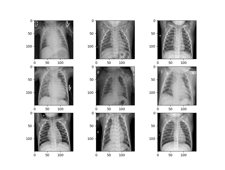
Let’s visualize some of the data to get a better idea of how the datasets will differ. First, we’ll visualize the data that is being used to train the first model.
def image_show(image_generator):
    x, y = image_generator.next()
    fig = plt.figure(figsize=(8, 8))
    columns = 3
    rows = 3
    for i in range(1, 10):
        # img = np.random.randint(10)
        image = x[i]
        fig.add_subplot(rows, columns, i)
        plt.imshow(image.transpose(0, 1, 2))
    plt.show()

image_show(train_generator_1)
Now we’ll visualize the second set of data.
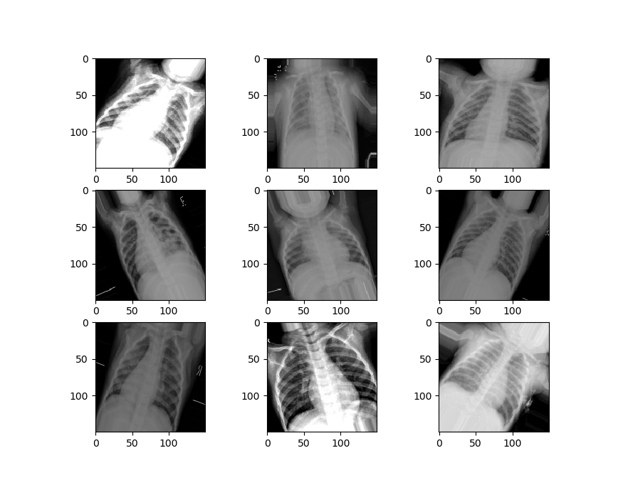
We can see that our second set of data is a little different from the first set. It’s zoomed in, rotated randomly, has image artifacts and more, to simulate the kinds of damages that might happen to an image in the real world.
Now we can make a function to handle the creation of our model. This function will establish the sequential model form and add the layers of the convolutional network – with the convolutional layers, the Max Pooling, and some batch normalization.
We’ll have three of these “blocks” comprising the convolutional layers in our network. These will be followed by a flattening layer, which transforms the data into a long vector that the densely connected layers of the neural network will be able to analyze. We’ll then add in our densely connected layers and activation functions, along with some dropout to prevent overfitting. We then compile the model and return it.
def create_model():
    # first specify the sequential nature of the model

    model = Sequential()

    # second parameter is the size of the "window" you want the CNN to use

    # the shape of the data we are passing in, 3 x 150 x 150
    # last element is just the image in the series, others are pixel widths

    model.add(Conv2D(64, (3, 3), input_shape=(150, 150, 3)))
    model.add(Activation("relu"))
    model.add(MaxPooling2D(pool_size=(2,2)))
    model.add(BatchNormalization())

    model.add(Conv2D(128, (3, 3)))
    model.add(Activation("relu"))
    model.add(MaxPooling2D(pool_size=(2,2)))
    model.add(BatchNormalization())

    model.add(Conv2D(256, (3, 3)))
    model.add(Activation("relu"))
    model.add(MaxPooling2D(pool_size=(2, 2)))
    model.add(BatchNormalization())

    model.add(Conv2D(256, (3, 3)))
    model.add(Activation("relu"))
    model.add(MaxPooling2D(pool_size=(2, 2)))
    model.add(BatchNormalization())

    # you'll need to flatten the data again if you plan on having Dense layers in the model,
    # as it needs a 1d unlike a 2d CNN

    model.add(Flatten())

    model.add(Dense(128, activation='relu'))
    model.add(Dropout(0.2))
    model.add(Dense(64, activation='relu'))
    model.add(Dropout(0.2))
    model.add(Dense(2, activation='sigmoid'))

    # now compile the model, specify loss, optimization, etc

    model.compile(loss='binary_crossentropy', optimizer='adam', metrics=['accuracy'])

    # fit the model, specify batch size, validation split and epochs

    return model

model = create_model()
Now we’ll create the model by calling the function.
We need to use the fit_generator function to fit our model since we used a data generator to set up the image data. We’re also going to specify some callbacks here, which specify how we want our model to behave while training.
The callbacks we will use include:
Model Checkpoint – which saves weights occasionally when a specified event happens (in our case when the validation accuracy improves.
Reduce LR On Plateau, which reduces the learning rate of our classifier when it hits a plateau and stops improving on the loss. This helps to avoid getting stuck oscillating around minimum loss.
Finally, Early Stopping lets us stop training early if we’ve hit a point where validation loss stops decreasing for some given amount of time, which is defined by our “patience”.
We pass in these callbacks and then fit the model, saving it in a variable so we can access the training records later.
filepath = "weights_training_1.hdf5"
callbacks = [ModelCheckpoint(filepath, monitor='val_acc', verbose=1, save_best_only=True, mode='max'),
              ReduceLROnPlateau(monitor='val_loss', factor=0.2, patience=3, verbose=1, mode='min', min_lr=0.00001),
              EarlyStopping(monitor= 'val_loss', min_delta=1e-10, patience=15, verbose=1, restore_best_weights=True)]

records = model.fit_generator(train_generator_1, steps_per_epoch=100, epochs=25, validation_data=test_generator_1, validation_steps=7, verbose=1, callbacks=callbacks)
After our training is complete and the best weights have been saved, let’s evaluate the performance of our model. We’ll create a function that plots the loss and accuracy of the training and validation sets. We’ll also evaluate the model’s performance using the evaluation metric we specified in the generator, which we can save to a variable and print.
First, we’ll need to get the loss on the training and validation sets, which we can draw from the “records” variable.
t_loss = records.history['loss']
v_loss = records.history['val_loss']
t_acc = records.history['acc']
v_acc = records.history['val_acc']

# gets the lengt of how long the model was trained for
train_length = range(1, len(t_acc) + 1)
Now we’ll create the function to evaluate our model’s performance.
def evaluation(model, train_length, training_acc, val_acc, training_loss, validation_loss, generator):

    # plot the loss across the number of epochs
    plt.figure()
    plt.plot(train_length, training_loss, label='Training Loss')
    plt.plot(train_length, validation_loss, label='Validation Loss')
    plt.xlabel('Epochs')
    plt.ylabel('Loss')
    plt.legend()

    plt.figure()
    plt.plot(train_length, training_acc, label='Training Accuracy')
    plt.plot(train_length, val_acc, label='Validation Accuracy')
    plt.title('Training and validation accuracy')
    plt.xlabel('Epochs')
    plt.ylabel('Accuracy')
    plt.legend()
    plt.show()

    # compare against the test training set
    # get the score/accuracy for the current model
    scores = model.evaluate_generator(generator)
    print("\n%s: %.2f%%" % (model.metrics_names[1], scores[1] * 100))
We have around 83% accuracy already. Not bad.
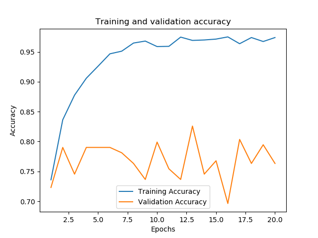
acc: 83.09%
Now we can call the function and evaluate how our model trained along with its performance on the dataset.
evaluation(model, train_length, t_acc, v_acc, t_loss, v_loss, test_generator_1)
We’re now going to train a second model that uses the weights and architecture from our first model. We’ll load in the trained weights into a second instance of our model. Then we’ll specify that we only want to train the last five layers of our model, a portion of the densely connected layers. We can make sure these are set up to train by printing out the trainable layers of the model.
model_2 = create_model()
model_2.load_weights("weights_training_1.hdf5")

for layer in model_2.layers[:-5]:
    layer.trainable = False

for layer in model_2.layers:
    print(layer, layer.trainable)
Now we just need to compile and fit the model.
# now compile the model, specify loss, optimization, etc
model_2.compile(loss='binary_crossentropy', optimizer='adam', metrics=['accuracy'])

# fit the model, specify batch size, validation split and epochs

filepath = "C:/Users/Daniel/Downloads/chest-xray-pneumonia/chest_xray/weights_training_2.hdf5"
callbacks = [ModelCheckpoint(filepath, monitor='val_acc', verbose=1, save_best_only=True, mode='max'),
              ReduceLROnPlateau(monitor='val_loss', factor=0.2, patience=3, verbose=1, mode='min', min_lr=0.00001),
              EarlyStopping(monitor= 'val_loss', min_delta=1e-10, patience=15, verbose=1, restore_best_weights=True)]

records = model_2.fit_generator(train_generator_2, steps_per_epoch=85, epochs=20, validation_data=test_generator_2, validation_steps=7, verbose=1, callbacks=callbacks)
Finally, let’s check to see how the second model performed by getting its metrics.
t_loss = records.history['loss']
v_loss = records.history['val_loss']
t_acc = records.history['acc']
v_acc = records.history['val_acc']

# gets the length of how long the model was trained for
train_length = range(1, len(t_acc) + 1)

evaluation(model_2, train_length, t_acc, v_acc, t_loss, v_loss, 80, test_generator_2)


acc: 73.48%
We can see that after training it for only two epochs, and despite the perturbations applied to the dataset, performance quickly hit over 70%.