After defining the functions we need, we’ll start off by loading in the data.
Afterwards, we’ll check to see if there’s any blank values.
import pandas as pd
import numpy as np

# check for missing data
def check_missing(dataframe, cols):

    for col in cols:
       print("Column {} is missing:".format(col))
       print((dataframe[col].values == ' ').sum())
       print()

# convert to numeric
def to_numeric(dataframe, cols):

    for col in cols:
        dataframe[col] = dataframe[col].convert_objects(convert_numeric=True)

# check frequency distribution
def freq_dist(dataframe, cols, norm_cols):

    for col in cols:
        print("Fred dist for: {}".format(col))
        count = dataframe[col].value_counts(sort=False, dropna=False)
        print(count)

    for col in norm_cols:
        print("Fred dist for: {}".format(col))
        count = dataframe[col].value_counts(sort=False, dropna=False, normalize=True)
        print(count)


df = pd.read_csv("gapminder.csv")

#print(dataframe.head())
print(df.isnull().values.any())

cols = ['lifeexpectancy', 'breastcancerper100th', 'suicideper100th']
norm_cols = ['internetuserate', 'employrate']

df2 = df.copy()

check_missing(df, cols)
check_missing(df, norm_cols)
There’s quite a few blank values:
22
Column breastcancerper100th is missing:
40
Column suicideper100th is missing:
22
Column internetuserate is missing:
21
Column employrate is missing:
35
Calling the to_numeric function should convert them into NaN values. Which we can check by calling the frequency distribution function.
to_numeric(df2, cols)
to_numeric(df2, norm_cols)
NaN 22
63.125 1
74.576 1
62.475 1
74.414 1
79.977 1
58.199 1
75.670 1
81.012 1
72.283 1
55.442 1
81.855 1
48.398 1
68.944 1
75.133 1
76.126 1
69.317 1
65.193 1
75.057 1
77.685 1
68.498 1
62.465 1
79.634 1
73.911 1
80.499 1
61.597 1
79.591 1
71.017 1
82.759 1
68.978 1
..
76.954 1
73.703 1
79.839 1
48.718 1
71.172 1
73.456 1
48.397 1
81.439 1
75.246 1
55.377 1
74.788 1
74.402 1
82.338 1
79.499 1
81.539 1
54.210 1
67.017 1
61.452 1
73.373 1
73.127 1
69.245 1
68.795 1
79.341 1
76.918 1
57.937 1
73.126 1
64.666 1
75.956 1
57.379 1
50.239 1
Name: lifeexpectancy, Length: 190, dtype: int64
Fred dist for: breastcancerper100th
23.5 2
NaN 40
70.5 1
31.5 1
62.5 1
36.0 1
92.0 1
46.0 1
19.5 6
21.5 1
16.5 3
26.0 1
29.5 1
63.0 1
90.0 1
43.5 1
33.0 1
23.0 1
52.5 1
30.6 1
38.5 1
82.5 1
10.5 1
22.5 2
90.8 1
29.0 1
55.5 1
48.0 1
35.0 1
25.2 1
..
58.9 2
23.3 1
33.4 1
28.1 7
29.7 1
83.2 1
84.3 1
50.1 1
43.9 1
4.4 1
19.6 1
29.8 2
17.3 2
18.7 1
31.2 3
20.6 2
38.7 1
21.8 2
58.4 2
35.1 2
24.2 1
13.6 1
30.3 1
18.2 2
79.8 1
46.2 1
62.1 1
50.4 2
46.6 1
31.7 1
Name: breastcancerper100th, Length: 137, dtype: int64
Fred dist for: suicideper100th
NaN 22
9.847460 1
6.519537 1
11.980497 1
13.716340 1
33.341860 1
2.034178 1
14.554677 1
6.449157 1
18.954570 1
5.554276 1
16.959240 1
10.493150 1
11.956941 1
4.961071 1
11.426181 1
4.930045 1
10.645740 1
11.655210 1
2.234896 1
2.515721 1
10.550375 1
1.658908 1
10.365070 1
8.164005 1
3.108603 1
16.234370 1
3.563325 1
10.100990 1
4.217076 1
..
15.538490 1
9.875281 1
10.171735 1
6.087671 1
5.838315 1
25.404600 1
13.637060 1
1.498057 1
8.283071 1
16.913248 1
27.874160 1
15.542603 1
5.767406 1
9.127511 1
4.288574 1
6.882952 1
12.405918 1
10.114997 1
7.699330 1
10.129350 1
13.548420 1
12.289122 1
20.369590 1
8.211067 1
3.716739 1
9.507928 1
2.109414 1
13.089616 1
9.257976 1
6.811439 1
Name: suicideper100th, Length: 192, dtype: int64
Fred dist for: internetuserate
81.000000 0.004695
66.000000 0.004695
45.000000 0.004695
NaN 0.098592
2.100213 0.004695
65.000000 0.004695
80.000000 0.004695
5.001375 0.004695
51.914184 0.004695
42.984580 0.004695
25.000000 0.004695
39.820178 0.004695
9.999954 0.004695
44.989947 0.004695
2.300027 0.004695
5.999836 0.004695
71.849124 0.004695
44.001025 0.004695
7.232224 0.004695
90.703555 0.004695
1.259934 0.004695
69.339971 0.004695
35.850437 0.004695
26.477223 0.004695
2.199998 0.004695
16.780037 0.004695
40.122235 0.004695
15.999650 0.004695
70.028599 0.004695
81.590397 0.004695
…
2.699966 0.004695
12.006692 0.004695
1.280050 0.004695
74.247572 0.004695
28.731883 0.004695
81.338393 0.004695
43.366498 0.004695
6.497924 0.004695
65.387786 0.004695
12.500255 0.004695
47.867469 0.004695
12.349750 0.004695
43.055067 0.004695
40.650098 0.004695
45.986590 0.004695
54.992809 0.004695
33.382128 0.004695
65.808554 0.004695
44.570074 0.004695
7.499996 0.004695
88.770254 0.004695
1.700031 0.004695
4.170136 0.004695
56.300034 0.004695
51.280478 0.004695
36.000335 0.004695
41.000128 0.004695
33.616683 0.004695
60.119707 0.004695
1.699985 0.004695
Name: internetuserate, Length: 193, dtype: float64
Fred dist for: employrate
50.500000 0.004695
NaN 0.164319
61.500000 0.014085
46.000000 0.009390
64.500000 0.004695
63.500000 0.004695
51.000000 0.009390
68.000000 0.004695
56.000000 0.009390
56.500000 0.004695
59.000000 0.009390
53.500000 0.014085
81.500000 0.004695
66.000000 0.009390
64.599998 0.004695
64.199997 0.004695
83.000000 0.004695
60.500000 0.004695
42.500000 0.004695
54.500000 0.009390
77.000000 0.004695
42.000000 0.004695
65.000000 0.014085
61.700001 0.004695
50.900002 0.009390
61.000000 0.009390
66.199997 0.004695
57.900002 0.004695
76.000000 0.004695
49.500000 0.004695
…
63.700001 0.004695
52.700001 0.004695
78.900002 0.004695
70.400002 0.009390
71.699997 0.004695
41.599998 0.004695
80.699997 0.004695
54.599998 0.004695
42.799999 0.004695
50.700001 0.004695
57.200001 0.004695
66.800003 0.004695
54.400002 0.004695
63.099998 0.004695
63.900002 0.004695
55.099998 0.004695
67.300003 0.004695
44.799999 0.004695
64.300003 0.004695
47.099998 0.004695
41.099998 0.004695
44.299999 0.004695
62.400002 0.004695
51.299999 0.004695
79.800003 0.004695
58.599998 0.004695
63.799999 0.009390
63.200001 0.004695
65.599998 0.004695
68.300003 0.004695
The blank values have successfully been replaced with NaN. This is good because when we plot graphs later, we can just have Python ignore those NaN values. We’ve coded out the missing data with NaN.
I’ve also decided to experiment with bins. We’ll do one more thing and create five bins for our chosen features.
Here’s the code to do that:
def bin(dataframe, cols):
for col in cols:
new_col_name = "{}_bins".format(col)
dataframe[new_col_name] = pd.qcut(dataframe[col], 5, labels=["1-20%", "21 to 40%", "40 to 60%", "60 to 80%", "80 to 100%"])
df3 = df2.copy()
bin(df3, cols)
bin(df3, norm_cols)
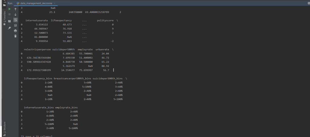
# print out the head and check the dataframe
print(df3.head())
Let’s print out the head of the dataframe to see if the values exist. It looks a little messy, but we can see that the new columns have successfully been created.