Investigating Religion and Poverty as They Relate to the Spread of Covid-19
There is a wealth of data online now regarding the number of Covid-19 cases in different regions of the world. Many of these datasets and accompanying analyses look at variables like population density and number of hospital beds in order to predict coronavirus case counts and death counts. I’d like to examine less commonly examined variables like religion and poverty and see if there are some potential correlations with spread (as measured by relative case counts) of Sars-Cov-2.
I hypothesize that both variables have some correlation with large gatherings of people and therefore could be tied to increased spread of coronavirus. For instance, more religious areas may have more gatherings due to church attendance while more poverty-stricken areas may hae more people rooming together to afford housing, and both could conceivably play a role in the spread of Sars-Cov-2. For that reason, I want to see if there are any correlations between these two variables and coronavirus case counts. I’d also like to see if these variables have any potential moderating effects on each other.
I think that finding potentially interesting correlations between these variables and the spread of Sars-Cov-2/coronavirus could help lay the groundwork for better understanding of how diseases like coronavirus spread throughout populations.
These are the results of a clustering analysis run on the Gapminder dataset. The features used to generate the three classes/categories include: alcohol consumption, breast cancer rate, employ rate, internet use rate, life expectancy, and urbanization rate.
After preprocessing the data, which includes scaling the features, it is separated into a training and testing data sets.
from sklearn.preprocessing import scale, MinMaxScaler
import pandas as pd
from seaborn import regplot
import matplotlib.pyplot as plt
import numpy as np
from sklearn.model_selection import train_test_split
from sklearn.cluster import KMeans
from scipy.spatial.distance import cdist
from sklearn.decomposition import PCA

import statsmodels.api as sm

# check for missing data
def check_missing(dataframe, cols):

    for col in cols:
       print("Column {} is missing:".format(col))
       print((dataframe[col].values == ' ').sum())
       print()

# convert to numeric
def to_numeric(dataframe, cols):

    for col in cols:
        dataframe[col] = pd.to_numeric(dataframe[col], errors='coerce')

# check frequency distribution
def freq_dist(dataframe, cols, norm_cols):

    for col in cols:
        print("Fred dist for: {}".format(col))
        count = dataframe[col].value_counts(sort=False, dropna=False)
        print(count)

    for col in norm_cols:
        print("Fred dist for: {}".format(col))
        count = dataframe[col].value_counts(sort=False, dropna=False, normalize=True)
        print(count)


df = pd.read_csv("gapminder.csv")

#print(dataframe.head())
#print(df.isnull().values.any())

cols = ['lifeexpectancy', 'breastcancerper100th', 'suicideper100th']
norm_cols = ['internetuserate', 'employrate', 'incomeperperson']

df2 = df.copy()

to_numeric(df2, cols)
to_numeric(df2, norm_cols)

df_clean = df2.dropna()

def plot_regression(x, y, data, label_1, label_2):

    reg_plot = regplot(x=x, y=y, fit_reg=True, data=data)
    plt.xlabel(label_1)
    plt.ylabel(label_2)
    plt.show()

def group_incomes(row):
    if row['incomeperperson'] <= 744.23:
        return 1
    elif row['incomeperperson'] <= 942.32:
        return 2
    else:
        return 3

df_clean['income_group'] = df_clean.apply(lambda row: group_incomes(row), axis=1)

scaler = MinMaxScaler()

X = df_clean[['alcconsumption','breastcancerper100th','employrate', 'internetuserate','lifeexpectancy','urbanrate']]
X.astype(float)

#print(X["internetuserate"].mean(axis=0))

X['internetuserate_scaled'] = scale(X['internetuserate'])
X['urbanrate_scaled'] = scale(X['urbanrate'])
X['lifeexpectancy_scaled'] = scale(X['lifeexpectancy'])
X['employrate_scaled'] = scale(X['employrate'])
X['alconsumption'] = scale(X['alcconsumption'])
X['breastcancerper100th'] = scale(X['breastcancerper100th'])

#print(X['internetuserate'].mean(axis=0))
#print(X['internetuserate_scaled'].mean(axis=0))

X_train, X_test = train_test_split(X, test_size=0.25)
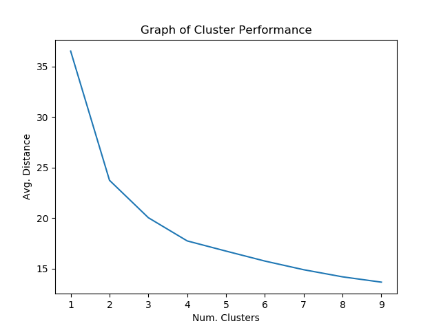
Afterwards, the model is tested on the dataset to determine which number of clusters seems to give the best performance.
clusters = range(1, 10) mean_dist = []
for i in clusters: model = KMeans(n_clusters=i) model.fit(X_train) clus_assign = model.predict(X_train) mean_dist.append(sum(np.min(cdist(X_train, model.cluster_centers_, 'euclidean'), axis=1))/X_train.shape[0])
Around 4 clusters seems to give the best results that might guard against overfitting.
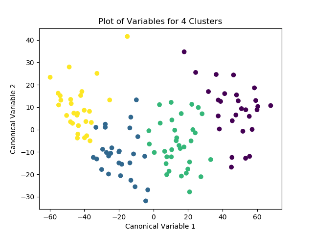
Afterwards, the model is run again with 4 clusters, this time with the PCA transformed variables passed in as the labels. After the optimized model is run, the means for the different classes are examined for meaningful patterns. The number of observations for each class is then distinguished and printed as the “cluster” variable. Finally, the means for the different clusters are calculated and the variable means for the different clusters can be explored.
K_means_model = KMeans(n_clusters=4)
K_means_model.fit(X_train)
clus_assign = K_means_model.predict(X_train)

pca_2 = PCA(2)
plot_columns = pca_2.fit_transform(X_train)
plt.scatter(x=plot_columns[:,0], y=plot_columns[:,1], c=K_means_model.labels_)
plt.xlabel("Canonical Variable 1")
plt.ylabel("Canonical Variable 2")
plt.title("Plot of Variables for 3 Clusters")
plt.show()

# check pattern of means by cluster to see if the means are distinct and meaningful
# create unique identifiers from the index of cluster training data
X_train.reset_index(level=0, inplace=True)
cluster_list = list(X_train['index'])
labels = list(K_means_model.labels_)
new_dict = dict(zip(cluster_list, labels))
print(new_dict)
new_cluster = pd.DataFrame.from_dict(new_dict, orient='index')
print(new_cluster)

# create unique identifiers for cluster assignment variable
# rename cluster assignment column
new_cluster.columns = ["cluster"]
new_cluster.reset_index(level=0, inplace=True)
merged_train = pd.merge(X_train, new_cluster, on='index')
print(merged_train.head(20))
print(merged_train.cluster.value_counts())

# we can now calculate means of variables for the different clusters
cluster_group = merged_train.groupby('cluster').mean()
print("Clustering variable means by cluster")
print(cluster_group)
Ignoring the index, we can look at some of the results for the column. It looks like, for example, observations in cluster 1 seem to have a higher likelihood of having high breast cancer rates compared to the other clusters. Meanwhile, observations in cluster 2 tended to have much lower alcohol consumption rates than average.
I ran a logistic regression on the Gapminder dataset. I chose to explore the relationship between life expectancy and internet use rate, as potentially moderated by employment rate. My hypothesis is that there is a positive correlation between life expectancy and internet use rate.
First, we’ll examine the relationship between life expectancy and internet use rate. After binning the life expectancy into two different categories, we can run the first logistic regression model.
from sklearn.preprocessing import scale, MinMaxScaler import statsmodels.formula.api as smf from scipy.stats import pearsonr import pandas as pd from seaborn import regplot import matplotlib.pyplot as plt import numpy as np
import statsmodels.api as sm
# check for missing data def check_missing(dataframe, cols):
for col in cols: print("Column {} is missing:".format(col)) print((dataframe[col].values == ' ').sum()) print()
# convert to numeric def to_numeric(dataframe, cols):
for col in cols: dataframe[col] = pd.to_numeric(dataframe[col], errors='coerce')
# check frequency distribution def freq_dist(dataframe, cols, norm_cols):
for col in cols: print("Fred dist for: {}".format(col)) count = dataframe[col].value_counts(sort=False, dropna=False) print(count)
for col in norm_cols: print("Fred dist for: {}".format(col)) count = dataframe[col].value_counts(sort=False, dropna=False, normalize=True) print(count)
The results of the first model show that there’s a fairly large P-value of approximately 0.50, implying that there’s no significant relationship between life expectancy and internet use rate. The odds ratio of approximately 0.99 shows that between the two groups (shorter lives and longer lives), the rate of internet use seems to be approximately equivalent. It’s 95% certain that the true population odds ratios fall somewhere between 0.97 and 1.01. It looks like the results of the logistic regression model do not support my hypothesis.
After running the first regression model, I ran another model that checked for possible confounding from the “employment rate” variable.
                           Logit Regression Results
===============================================================================
Dep. Variable:     lifeexpectancy_bins   No. Observations:                  167
Model:                           Logit   Df Residuals:                      164
Method:                            MLE   Df Model:                            2
Date:                 Mon, 25 May 2020   Pseudo R-squ.:                  0.3124
Time:                         01:40:11   Log-Likelihood:                -22.081
converged:                        True   LL-Null:                       -32.114
Covariance Type:             nonrobust   LLR p-value:                 4.393e-05
===================================================================================
                      coef    std err          z      P>|z|      [0.025      0.975]
-----------------------------------------------------------------------------------
Intercept          -1.3109      2.402     -0.546      0.585      -6.018       3.396
internetuserate     0.2311      0.105      2.209      0.027       0.026       0.436
employrate          0.0320      0.035      0.919      0.358      -0.036       0.100
===================================================================================

Possibly complete quasi-separation: A fraction 0.41 of observations can be
perfectly predicted. This might indicate that there is complete
quasi-separation. In this case some parameters will not be identified.
Odd ratio:
Intercept          0.269569
internetuserate    1.259940
employrate         1.032473
dtype: float64
Confidence intervals:
                 Lower CI   Upper CI        OR
Intercept        0.002434  29.851462  0.269569
internetuserate  1.026374   1.546656  1.259940
employrate       0.964467   1.105275  1.032473
When this second regression model was run, it was found that there does seem to be a significant relationship between life expectancy and internet use rate, as this second model returned a P-value of 0.027 for internet use rate. Meanwhile, the P-value of employment rate was approximately 0.35, indicating a non-significant relationship. That said, the relationship appears to be a fairly weak one, with countries with high internet use rates are only about 1.25 times more likely to have long life expectancies than countries without high internet use rates. In terms of employment rates, the odds ratio is very near 1 (1.03), which implies a non-significant relationship between employment rates and life expectancy. The results suggest that employment rates confound the relationship between internet use rates and life expectancy.
I’ll be carrying out lasso regression on the Gapminder dataset. The features we are investigating are the following: “alcohol consumption”, “breast cancer per 100k”, “employment rate”, “internet use rate”, “life expectancy”, and “urbanization rate”. We are hoping to predict which income group the data points (countries) fall into based on the provided features.
First, we’ll need to load in the data and preprocesss the data, scaling the features of interest.
from sklearn.preprocessing import scale, MinMaxScaler
import statsmodels.formula.api as smf
from scipy.stats import pearsonr
import pandas as pd
from seaborn import regplot
import matplotlib.pyplot as plt
import statsmodels.api as sm
from sklearn.linear_model import LassoLarsCV
from sklearn.model_selection import train_test_split
from sklearn.metrics import mean_squared_error

# check for missing data
def check_missing(dataframe, cols):

    for col in cols:
       print("Column {} is missing:".format(col))
       print((dataframe[col].values == ' ').sum())
       print()

# convert to numeric
def to_numeric(dataframe, cols):

    for col in cols:
        dataframe[col] = dataframe[col].convert_objects(convert_numeric=True)

# check frequency distribution
def freq_dist(dataframe, cols, norm_cols):

    for col in cols:
        print("Fred dist for: {}".format(col))
        count = dataframe[col].value_counts(sort=False, dropna=False)
        print(count)

    for col in norm_cols:
        print("Fred dist for: {}".format(col))
        count = dataframe[col].value_counts(sort=False, dropna=False, normalize=True)
        print(count)


df = pd.read_csv("gapminder.csv")

cols = ['lifeexpectancy', 'breastcancerper100th', 'suicideper100th']
norm_cols = ['internetuserate', 'employrate', 'incomeperperson']

df2 = df.copy()

to_numeric(df2, cols)
to_numeric(df2, norm_cols)

df_clean = df2.dropna()

def plot_regression(x, y, data, label_1, label_2):

    reg_plot = regplot(x=x, y=y, fit_reg=True, data=data)
    plt.xlabel(label_1)
    plt.ylabel(label_2)
    plt.show()

def group_incomes(row):
    if row['incomeperperson'] <= 744.23:
        return 1
    elif row['incomeperperson'] <= 942.32:
        return 2
    else:
        return 3

df_clean['income_group'] = df_clean.apply(lambda row: group_incomes(row), axis=1)

scaler = MinMaxScaler()

X = df_clean[['alcconsumption','breastcancerper100th','employrate', 'internetuserate','lifeexpectancy','urbanrate']]
X.astype(float)

print(X["internetuserate"].mean(axis=0))


X['alcconsumption'] = scale(X['alcconsumption'])
X['breastcancerper100th'] = scale(X['breastcancerper100th'])
X['internetuserate'] = scale(X['internetuserate'])
X['urbanrate'] = scale(X['urbanrate'])
X['lifeexpectancy'] = scale(X['lifeexpectancy'])
X['employrate'] = scale(X['employrate'])

print(X['internetuserate'].mean(axis=0))

X.astype(float)
Y = df_clean['income_group']
Y.astype(float)
No features were dropped by the Lasso regression model. Life Expectancy and Urbanization rate appeared to have the strongest associations with income level.
Accuracy on the test dataset was around 66%, which is better than chance guessing but still leaves much room for improvement. Adding more features to the model would probably improve the model’s estimation accuracy. In terms of the R-squared, the model performed just slightly better on the training dataset, explaining approximately 60% of the variance in the training dataset, contrasted with the approx. 57% of the variance explained for the testing set.
I am running a multi-regression model on the Gapminder dataset. Our dependent variable under study is life expectancy, while the independent variables we are investigating are “internet use rate”, “urbanization rate”, and “employment rate”.
First, we’re going to load in the data and do any necessary preprocessing of the dataset. This includes scaling the features of interest.
from sklearn.preprocessing import scale, MinMaxScaler
import statsmodels.formula.api as smf
from scipy.stats import pearsonr
import pandas as pd
from seaborn import regplot
import matplotlib.pyplot as plt
import statsmodels.api as sm

# check for missing data
def check_missing(dataframe, cols):

    for col in cols:
       print("Column {} is missing:".format(col))
       print((dataframe[col].values == ' ').sum())
       print()

# convert to numeric
def to_numeric(dataframe, cols):

    for col in cols:
        dataframe[col] = dataframe[col].convert_objects(convert_numeric=True)

# check frequency distribution
def freq_dist(dataframe, cols, norm_cols):

    for col in cols:
        print("Fred dist for: {}".format(col))
        count = dataframe[col].value_counts(sort=False, dropna=False)
        print(count)

    for col in norm_cols:
        print("Fred dist for: {}".format(col))
        count = dataframe[col].value_counts(sort=False, dropna=False, normalize=True)
        print(count)


df = pd.read_csv("gapminder.csv")

#print(dataframe.head())
#print(df.isnull().values.any())

cols = ['lifeexpectancy', 'breastcancerper100th', 'suicideper100th']
norm_cols = ['internetuserate', 'employrate', 'incomeperperson']

df2 = df.copy()

to_numeric(df2, cols)
to_numeric(df2, norm_cols)

df_clean = df2.dropna()

def plot_regression(x, y, data, label_1, label_2):

    reg_plot = regplot(x=x, y=y, fit_reg=True, data=data)
    plt.xlabel(label_1)
    plt.ylabel(label_2)
    plt.show()

def group_incomes(row):
    if row['incomeperperson'] <= 744.23:
        return 1
    elif row['incomeperperson'] <= 942.32:
        return 2
    else:
        return 3

df_clean['income_group'] = df_clean.apply(lambda row: group_incomes(row), axis=1)

scaler = MinMaxScaler()

X = df_clean[['alcconsumption','breastcancerper100th','employrate', 'internetuserate','lifeexpectancy','urbanrate']]
X.astype(float)

print(X["internetuserate"].mean(axis=0))

X['internetuserate_scaled'] = scale(X['internetuserate'])
X['urbanrate_scaled'] = scale(X['urbanrate'])
X['lifeexpectancy_scaled'] = scale(X['lifeexpectancy'])
X['employrate_scaled'] = scale(X['employrate'])

print(X['internetuserate'].mean(axis=0))
print(X['internetuserate_scaled'].mean(axis=0))
Now that we’ve scaled the features, we can run a multiple linear regression on the chosen features. We’ll also visualize the results of the residuals by creating some plots. We’ll create a QQ plot, a residual plot, and a influence/leverage plot.
1) Discuss the results for the associations between all of your explanatory variables and your response variable. Make sure to include statistical results (Beta coefficients and p-values) in your summary.
The response variable is Life Expectancy, while the explanatory varaibles are Internet Use Rate, Urbanization Rate, and Employment rate. All three explanatory variables seem to have a signficant P-value, with a P-value of ~0, 0.003, and 0.012 for InternetUseRate, UrbanRate, and EmployRate respectively. Checking the beta coefficients for the three explanatory variables gives us some insight into the degrees of change for the three variables. InternetUseRate has a coefficient of approximately 0.60. Meanwhile, UrbanRate has about a third of the relationship strength that InternetUseRate does. Employrate seems to have a slightly negative relationship with the response variable when checking just the coefficient, though if the two variables are graphed it shows that it has a non-linear, parabolic relationship.
2) Report whether your results supported your hypothesis for the association between your primary explanatory variable and the response variable.
The hypothesis was that internet use rate was positively correlated with life expectancy, and the multiple regression model seems to support this hypothesis.
3) Discuss whether there was evidence of confounding for the association between your primary explanatory and response variable (Hint: adding additional explanatory variables to your model one at a time will make it easier to identify which of the variables are confounding variables);
As none of the three tested variables had a P-value of greater than 0.05, it doesn’t seem that there is any evidence of confounding variables.
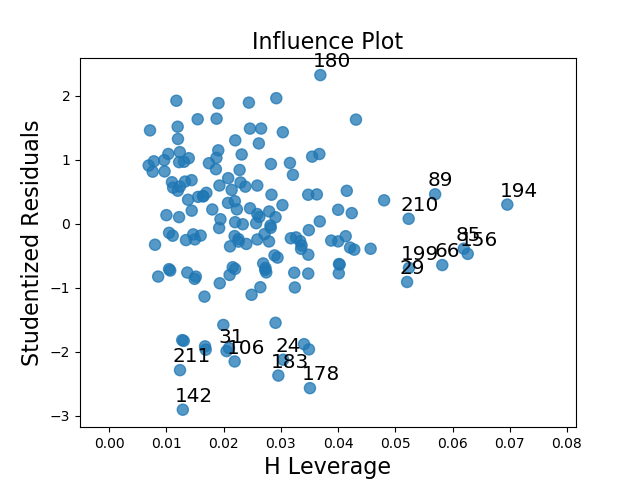
4) Generate the following regression diagnostic plots:
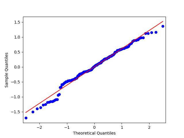
a) q-q plot
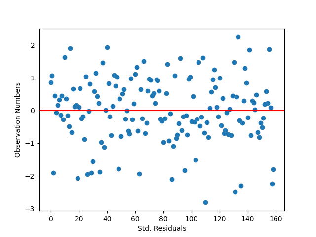
b) standardized residuals for all observations
c) leverage plot
d) Write a few sentences describing what these plots tell you about your regression model in terms of the distribution of the residuals, model fit, influential observations, and outliers.
The QQ plot indicates that there is a fairly tight fit to the distribution line, though the points deviate off of it at the lower and upper ends. This seems to indicate that the data is roughly normally distributed, but not perfectly normally distributed. Including other, higher order, variables in the regression model might help better capture the relationship.
The standardized residual graph shows that the vast majority of instances in the dataset have residuals that fall within two standard deviations from the mean, which fits the expectations for a normal distribution. It doesn’t look like any data points fall outside of three standard deviations from the mean, though there are some potential outliers. The model’s fit could potentially be improved by adding in new variables that might impact the relationships with the dependent variable.
The leverage plot suggests that there are a handful of outliers that have a notable, though not overwhelming, influence on the model’s estimations (points 183, 178, and 180). There also appear to be some instances which have a powerful impact on the model’s estimations, though in general they are not outliers as they do not fall outside of 1 standard deviation from the mean (the cluster on the far right of the graph).
We’ll be running a Random Forest classifier on the Gapminder dataset. Using a handful of variables to predict income levels, which have been grouped into three different levels.
We’ll start by loading in the data, preprocessing the data, and creating a new feature is the income level divided into three different groups.
from sklearn.model_selection import train_test_split
from sklearn.ensemble import RandomForestClassifier
from sklearn.metrics import confusion_matrix, accuracy_score
from scipy.stats import pearsonr
import pandas as pd
from seaborn import regplot
import matplotlib.pyplot as plt

# check for missing data
def check_missing(dataframe, cols):

for col in cols:
print("Column {} is missing:".format(col))
print((dataframe[col].values == ' ').sum())
print()

# convert to numeric
def to_numeric(dataframe, cols):

for col in cols:
dataframe[col] = dataframe[col].convert_objects(convert_numeric=True)

# check frequency distribution
def freq_dist(dataframe, cols, norm_cols):

for col in cols:
print("Fred dist for: {}".format(col))
count = dataframe[col].value_counts(sort=False, dropna=False)
print(count)

for col in norm_cols:
print("Fred dist for: {}".format(col))
count = dataframe[col].value_counts(sort=False, dropna=False, normalize=True)
print(count)


df = pd.read_csv("gapminder.csv")

#print(dataframe.head())
#print(df.isnull().values.any())

cols = ['lifeexpectancy', 'breastcancerper100th', 'suicideper100th']
norm_cols = ['internetuserate', 'employrate', 'incomeperperson']

df2 = df.copy()

#check_missing(df, cols)
#check_missing(df, norm_cols)

to_numeric(df2, cols)
to_numeric(df2, norm_cols)

#freq_dist(df2, cols, norm_cols)

df_clean = df2.dropna()


def plot_regression(x, y, data, label_1, label_2):

reg_plot = regplot(x=x, y=y, fit_reg=True, data=data)
plt.xlabel(label_1)
plt.ylabel(label_2)
plt.show()

print('Association between life expectancy and internet use rate')
print(pearsonr(df_clean['lifeexpectancy'], df_clean['internetuserate']))

print('Association between employment rate and internet use rate')
print(pearsonr(df_clean['employrate'], df_clean['internetuserate']))

def group_incomes(row):
if row['incomeperperson'] <= 744.23:
return 1
elif row['incomeperperson'] <= 942.32:
return 2
else:
return 3

df_clean['income_group'] = df_clean.apply(lambda row: group_incomes(row), axis=1)
We’ll now use the Train-Test split function to divide the dataset into training and testing sets. After this, we’ll fit the classifier, get predictions and print some statistics about the performance of the model.
X = df_clean[['alcconsumption','breastcancerper100th','employrate', 'internetuserate','lifeexpectancy','urbanrate']] X.astype(float) Y = df_clean['income_group'] Y.astype(float)
X_train, X_test, y_train, y_test = train_test_split(X, Y, test_size=0.25)
We’ll be running a basic linear regression on the Gapminder dataset. To begin with, we’ll start by importing all the necessary libraries and transforming the data.
from sklearn.preprocessing import scale, MinMaxScaler
import statsmodels.formula.api as smf
from scipy.stats import pearsonr
import pandas as pd
from seaborn import regplot
import matplotlib.pyplot as plt

# check for missing data
def check_missing(dataframe, cols):

    for col in cols:
       print("Column {} is missing:".format(col))
       print((dataframe[col].values == ' ').sum())
       print()

# convert to numeric
def to_numeric(dataframe, cols):

    for col in cols:
        dataframe[col] = dataframe[col].convert_objects(convert_numeric=True)

# check frequency distribution
def freq_dist(dataframe, cols, norm_cols):

    for col in cols:
        print("Fred dist for: {}".format(col))
        count = dataframe[col].value_counts(sort=False, dropna=False)
        print(count)

    for col in norm_cols:
        print("Fred dist for: {}".format(col))
        count = dataframe[col].value_counts(sort=False, dropna=False, normalize=True)
        print(count)


df = pd.read_csv("gapminder.csv")

#print(dataframe.head())
#print(df.isnull().values.any())

cols = ['lifeexpectancy', 'breastcancerper100th', 'suicideper100th']
norm_cols = ['internetuserate', 'employrate', 'incomeperperson']

df2 = df.copy()

#check_missing(df, cols)
#check_missing(df, norm_cols)

to_numeric(df2, cols)
to_numeric(df2, norm_cols)

#freq_dist(df2, cols, norm_cols)

df_clean = df2.dropna()

def plot_regression(x, y, data, label_1, label_2):

    reg_plot = regplot(x=x, y=y, fit_reg=True, data=data)
    plt.xlabel(label_1)
    plt.ylabel(label_2)
    plt.show()

print('Association between life expectancy and internet use rate')
print(pearsonr(df_clean['lifeexpectancy'], df_clean['internetuserate']))

print('Association between employment rate and internet use rate')
print(pearsonr(df_clean['employrate'], df_clean['internetuserate']))

def group_incomes(row):
    if row['incomeperperson'] <= 744.23:
        return 1
    elif row['incomeperperson'] <= 942.32:
        return 2
    else:
        return 3

df_clean['income_group'] = df_clean.apply(lambda row: group_incomes(row), axis=1)

#print(df_clean.head())
Now let’s check create an instance of the Scaler from Scikit-learn.
scaler = MinMaxScaler()

X = df_clean[['alcconsumption','breastcancerper100th','employrate', 'internetuserate','lifeexpectancy','urbanrate']]
X.astype(float)
We’ll now check the mean before we center/scale the data and after we do the scaling.
The first regression finds that there is a very strong relationship between the two variables, with an extremely small P-value of 1.77e-32. Meanwhile, the second set of variables still has a fairly strong, though not as strong, relationship as indicated by the P-value of 0.0120.
Meanwhile, the target variable is the income group that was created in the lesson on confounding variable comparisons.
Here’s the shape of the training and testing datasets:
(127, 6) (127,) (32, 6) (32,)
Here’s the accuracy for the decision tree:
0.8125
And here’s the confusion matrix: [[ 8 0 2] [ 1 0 0] [ 3 0 18]]
The correct predictions can be found running diagonally from the top left to the bottom right. It looks like the model was able to guess 8 instances in Group 1 correctly, 0 in Group 2, and 18 in Group 3. The model seems to be weakest at classifying Group 2 instances. Adding more explanatory variables other than the ones I have selected would likely help improve the model’s predictive power.
We’re going to be checking to see if income level might have any effect on the relationship between internet usage rates and life expectancy.
Here’s the code used to carry out the check for moderators.
from scipy.stats import pearsonr import pandas as pd from seaborn import regplot import matplotlib.pyplot as plt import numpy as np
# check for missing data def check_missing(dataframe, cols):
for col in cols: print("Column {} is missing:".format(col)) print((dataframe[col].values == ' ').sum()) print()
# convert to numeric def to_numeric(dataframe, cols):
for col in cols: dataframe[col] = dataframe[col].convert_objects(convert_numeric=True)
# check frequency distribution def freq_dist(dataframe, cols, norm_cols):
for col in cols: print("Fred dist for: {}".format(col)) count = dataframe[col].value_counts(sort=False, dropna=False) print(count)
for col in norm_cols: print("Fred dist for: {}".format(col)) count = dataframe[col].value_counts(sort=False, dropna=False, normalize=True) print(count)
print('Association between life expectancy and internet use rate for low income countries') print(pearsonr(subframe_1['lifeexpectancy'], subframe_1['internetuserate'])) print('Association between life expectancy and internet use rate for medium income countries') print(pearsonr(subframe_2['lifeexpectancy'], subframe_2['internetuserate'])) print('Association between life expectancy and internet use rate for high income countries') print(pearsonr(subframe_3['lifeexpectancy'], subframe_3['internetuserate']))
Three different income groups are created using a lambda function and the “group_incomes” function.
Here are the results of the code:
Association between life expectancy and internet use rate for low income countries (0.38386370068495235, 0.010101223355274047) Association between life expectancy and internet use rate for medium income countries (0.9966009508278395, 0.05250454954743393) Association between life expectancy and internet use rate for high income countries (0.7019997488251704, 6.526819886007788e-18)
For low income countries, there is a moderate correlation between life expectancy and internet use rate, with a small P-value. For middle income countries, the correlation is very strong, but the P-value is too large to be considered significant. For high income countries, the correlation is decently strong with a very small P-value, suggesting a significant correlation.
This is a summary of the GapMinder data and the chosen attributes/features for the analysis project.
Step 1: Describe your sample.
The dataset I am using is the GapMinder data, collected by the GapMinder foundation (created by Ola Rosling, Anna Rosling Rönnlund and Hans Rosling). The GapMinder dataset includes demographic data for all 192 member states of the United Nations as well as 24 other geographical regions.
The populations studies in the GapMinder data are the populations of the 215 geographic regions, and the level of analysis is the population of that region/aggregate statistics on that population. There are 215 observations in the dataset, the 192 UN members + 24 other regions. I am using all 215 observations in the dataset for my analysis, examining trends in their populations.
Step 2: Describe the procedures that were used to collect the data.
The GapMinder dataset contains information about a variety of population metrics like income per person, CO-2 emissions, employment rates, internet use rate, and life expectancy. This data was collected from a variety of sources such as the US Census Bureau’s International Database, the World Bank, and the United Nations Statistics Division. They were mainly collected through data reporting and surveys. The data was collected from 2002 to 2011, aggregated trough government reports and surveys done by independent organizations like the World Bank. The data was collected across the 215 geographical regions mentioned above.
Step 3: Describe your variables.
I’m curious to see if there might be some relationship between internet use rate and life expectancy, or beyond that if there might be a relationship between internet use rate and employment rate. This means that the explanatory variable is internet use rate and it tracks the percentage of a country’s population that has access to the internet. Meanwhile, life expectancy tracks the the average lifetime of a person within the various countries and employment rate tracks the percentage of a population that are employed. The scales for internet use rate and employment rate run from 0 to 100%, while life expectancy begins at 0 and runs upwards with an upper bound of approximately 82 years. The explanatory and response variables were made numeric and any blanks were replaced with NaN values.